createEPMgrid, the options
On this page, we will look more closely at all of the options that exist in the createEPMgrid() function, and provide examples when possible.
There are two options for determining whether a species range polygon should register in a given grid cell.
- With method 'centroid', a range polygon registers if it intersects the centroid coordinates of the grid cell.
- With method 'percentOverlap', a range polygon registers for a given cell if it covers xx% of that cell, where xx is supplied via the 'percentThreshold' input argument.
The difference between these two approaches is best demonstrated with an example:
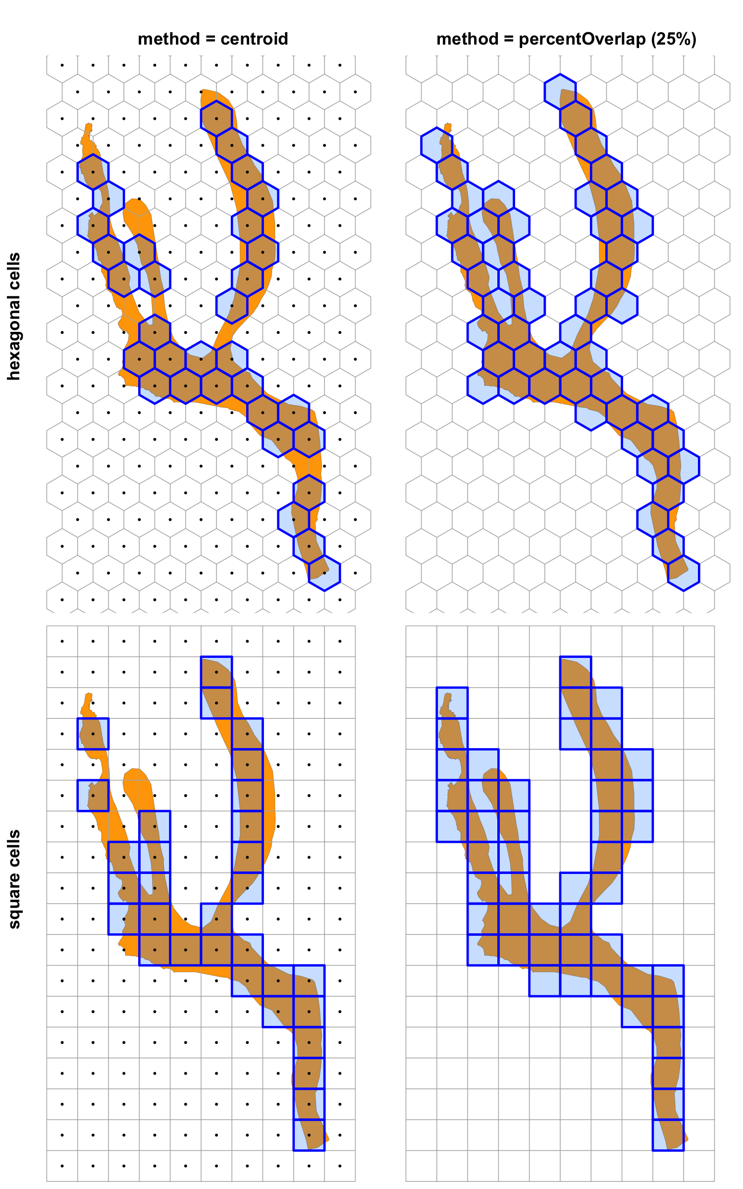
Which method is preferable will depend on the use-case scenario, where one approach may be more reasonable than the other. At coarse spatial scales, it is perhaps more likely that a species range polygon will be "missed" by cell centroid coordinates if those centroids are far apart from one another, something that will be less likely to be a problem if percent cover is the approach that is used. As the resolution of the grid increases, these differences will become increasingly minor.
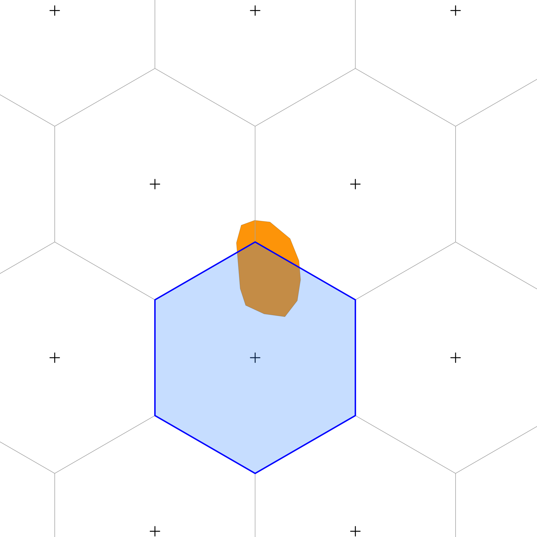
Species that inhabit small geographic ranges, such as microendemics, may not register in any grid cell, depending on the spatial resolution and the method used, and would therefore get dropped. This could happen if the entirety of these geographic ranges avoid all gridcell centroids (with method = 'centroid'), or if the species range occupies an area below the threshold for inclusion (if method = 'areaCutoff'). However, such small-ranged species may be particularly important for the analysis that is being undertaken. Therefore, there is an option that exists to force these species to be retained in the epmGrid object. If this option is enabled, then the single grid cell that is most occupied by the small-ranged species will register the species as present.
In the following example, with a grid system resolution of 50km, a species with a geographic range spanning 300 km2 would normally not register in any grid cell, as it does not intersect any centroid coordinates, nor does it cover 10% of any cell. If retainSmallRanges = TRUE, then the cell that most intersects the polygon will record the species as present. Only a single cell is recorded, so as to avoid small ranged species registering in multiple large cells, despite barely overlapping with those cells.
The createEPMgrid() function allows you to supply information on the extent in a number of ways:
- If
extent = 'auto', then all input data are examined, and the minimum bounding box that contains all species ranges is used. - A vector of values in the form of
c(minX, maxX, minY, maxY)can be provided, which would specify the bounding box for the extent. - A polygon of class sf or SpatialPolygons can be supplied to the extent argument. In this case, not only is the bounding box of that polygon used, but the epmGrid object is masked to that polygon (i.e., grid cells within the bounding box but outside of the polygon will be ignored).
- A raster of class SpatRaster or RasterLayer can be supplied to the extent argument. The bounding coordinates will be derived from this raster object (but nothing else, unlike with the use of
template, see below). - Interactively, where you will be provided the opportunity to draw your own extent.
See the following examples, using the built-in chipmunk dataset, which includes a list of 24 Tamias species range polygons:
> library(epm)
> tamiasPolyList
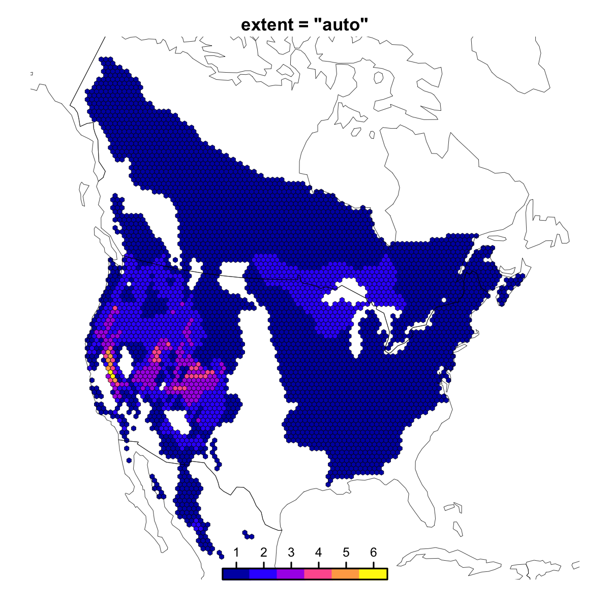
This (default) option is relatively straightforward. The extent is inferred directly from the input geographic data.
tamiasEPM <- createEPMgrid(tamiasPolyList, resolution = 50000, cellType = 'hexagon', method = 'centroid', extent = 'auto')

plot(tamiasEPM, use_tmap = FALSE, legend = FALSE)
mtext('extent = "auto"', font = 2, cex = 0.7)
addLegend(tamiasEPM, location = 'bottom', ramp = sf::sf.colors(100), ncolors = 6, cex.axis = 0.5, labelDist = 0.2)
With this option, horizontal and vertical extreme values can be provided to define a bounding box as extent. Note that this must be in the same map units as the input data.
minX <- -2e6
maxX <- 0
minY <- -1e6
maxY <- 2e6
bbVec <- c(minX, maxX, minY, maxY)

plot(tamiasEPM, use_tmap = FALSE, legend = FALSE)
abline(h=c(minY, maxY), lty = 2, lwd = 0.5, col = 'red')
abline(v = c(minX, maxX), lty = 2, lwd = 0.5, col = 'red')

tamiasEPM2 <- createEPMgrid(tamiasPolyList, resolution = 50000, cellType = 'hexagon', method = 'centroid', extent = bbVec)

plot(tamiasEPM2, use_tmap = FALSE, legend = FALSE)
mtext('extent = c(minX, maxX, minY, maxY)', font = 2, cex = 0.7)
addLegend(tamiasEPM2, location = 'bottom', ramp = sf::sf.colors(100), ncolors = 6, cex.axis = 0.5, labelDist = 0.2)
On the left, we've plotted lines to show what bounding values we've chosen. On the right is the resulting epmGrid object.
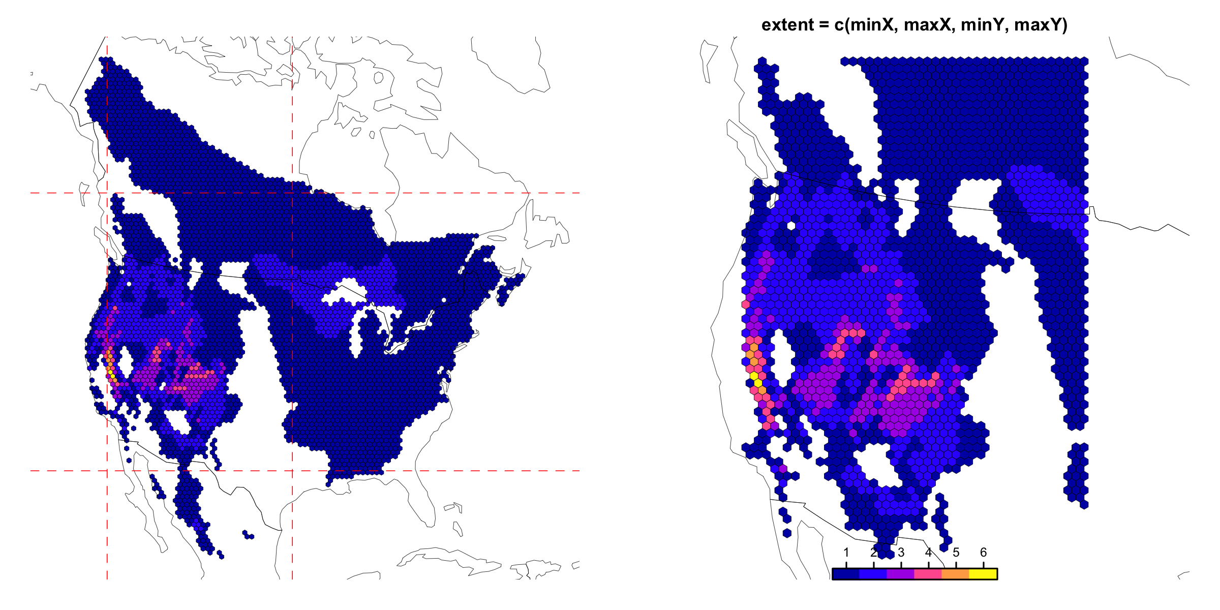
In this case, the epmGrid object will be limited to the extent of the supplied polygon. If the polygon is not a rectangle, then grid cells outside of the polygon but inside the bounding box will be ignored.
The polygon could be provided in any number of ways, via a shapefile read in from file, or from geospatial work done in R. Here, we will define a polygon according to a couple of vertices. Note that the vertex coordinates must be in the same units as the input species spatial data.
library(sf)

polyCoords <- rbind(c(-2267728, 2255199),
                    c(-635679.1, 1152463),
                    c(-238694.3, -2111634),
                    c(-1760469, -2133688),
                    c(-2708822, -259038.1),
                    c(-2267728, 2255199))

# (the last coordinate must be the same as the first coordinate to close the ring.)

# Convert table of coordinates into a polygon, specifying the same projection as the input species data.
bb <- st_sfc(st_polygon(list(polyCoords)), crs = st_crs(tamiasPolyList[[1]]))
(The polygon could also have been supplied as a SpatialPolygons object.)
par(mfrow = c(1,2))

# plot the full-extent epmGrid and overlay with the polygon we defined.
plot(tamiasEPM, use_tmap = FALSE, legend = FALSE)
plot(bb, add = TRUE, border = 'red', lwd = 2)

# Now use that polygon to constrain the extent.
tamiasEPM3 <- createEPMgrid(tamiasPolyList, resolution = 50000, cellType = 'hexagon', method = 'centroid', extent = bb)

plot(tamiasEPM3, use_tmap = FALSE, legend = FALSE)
mtext('extent = polygon', font = 2, cex = 0.7)
addLegend(tamiasEPM3, location = 'bottom', ramp = sf::sf.colors(100), ncolors = 6, cex.axis = 0.5, labelDist = 0.2)
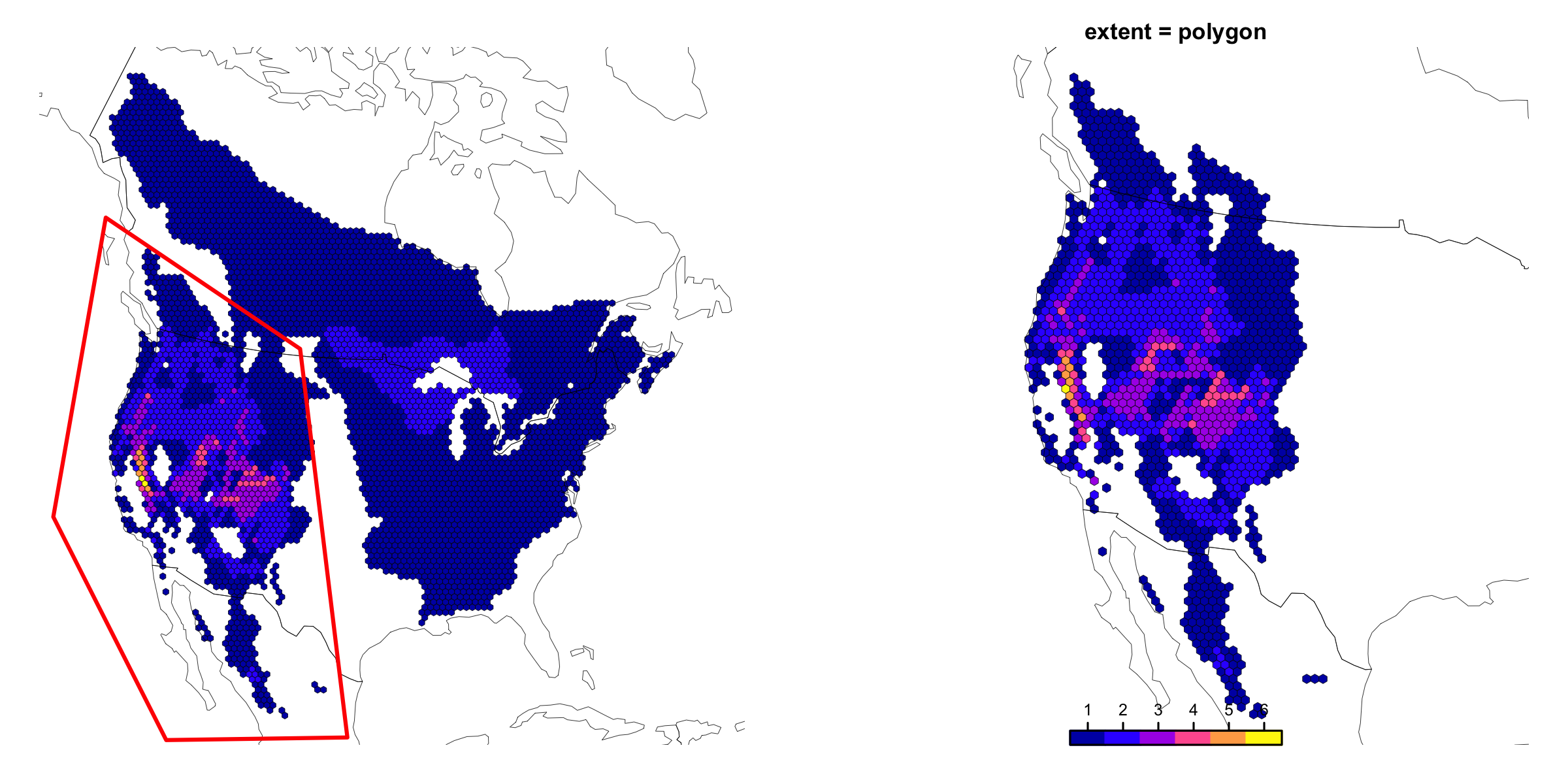
The function interactiveExtent is meant to provide a convenient way to specify the extent graphically, without needing to sort out what coordinates define the desired extent.
This is a two-step process:
- First, you run the
interactiveExtent()function, where a coarse-grained species richness map with the full extent is plotted, and you can then click on this map, and with each click you will draw a polygon. Right-clicking anywhere on the map will close the polygon and end the interactive plotting (or if in RStudio, click "finish"). This function call will return the polygon you drew, for future use. It will return your extent in two formats: As a sf polygon, and as a WKT string. A good strategy for maintaining reproducibility might be to copy/paste the WKT string that is returned into your R script. This way, you can read it back in and use it as the extent in the future. - You can then call the
createEPMgrid()function, but provide your extent to theextentargument.
Step 1: Interactively draw the extent polygon.
extentPoly <- interactiveExtent(tamiasPolyList)
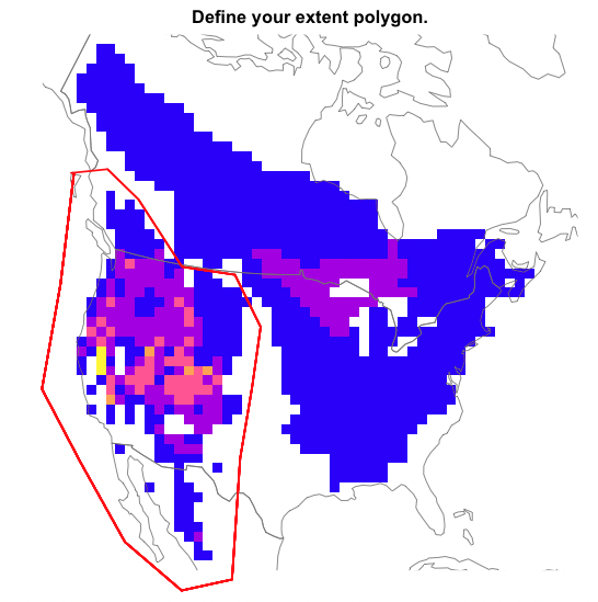
Be sure to direct this to a new variable name, as the drawn polygon will be returned:
> extentPoly$wkt
[1] "POLYGON ((-2266561 2100253, -2404525 964062.4, -2594908 -109635.3, -2198250 -862418.3, -1742016 -1679382, -1159302 -2177397, -641624.2 -2064408, -557927.7 -819279.7, -436133.7 -95659.28, -347627.5 527423.1, -611715.9 1062838, -1155296 1144978, -1603201 1837008, -1921257 2146497, -2295531 2107703, -2266561 2100253))"
This can be copy/pasted in your R script for future use and to ensure reproducibility:
extentPoly <- "POLYGON ((-2266561 2100253, -2404525 964062.4, -2594908 -109635.3, -2198250 -862418.3, -1742016 -1679382, -1159302 -2177397, -641624.2 -2064408, -557927.7 -819279.7, -436133.7 -95659.28, -347627.5 527423.1, -611715.9 1062838, -1155296 1144978, -1603201 1837008, -1921257 2146497, -2295531 2107703, -2266561 2100253))"
Step 2: Supply this drawn extent polygon directly to the extent argument.
tamiasEPM4 <- createEPMgrid(tamiasPolyList, resolution = 50000, cellType = 'hexagon', method = 'centroid', extent = extentPoly)

plot(tamiasEPM4, use_tmap = FALSE, legend = FALSE)
mtext('extent = drawn polygon', font = 2, cex = 0.7)
addLegend(tamiasEPM4, location = 'bottom', ramp = sf::sf.colors(100), cex.axis = 0.5, labelDist = 0.2)
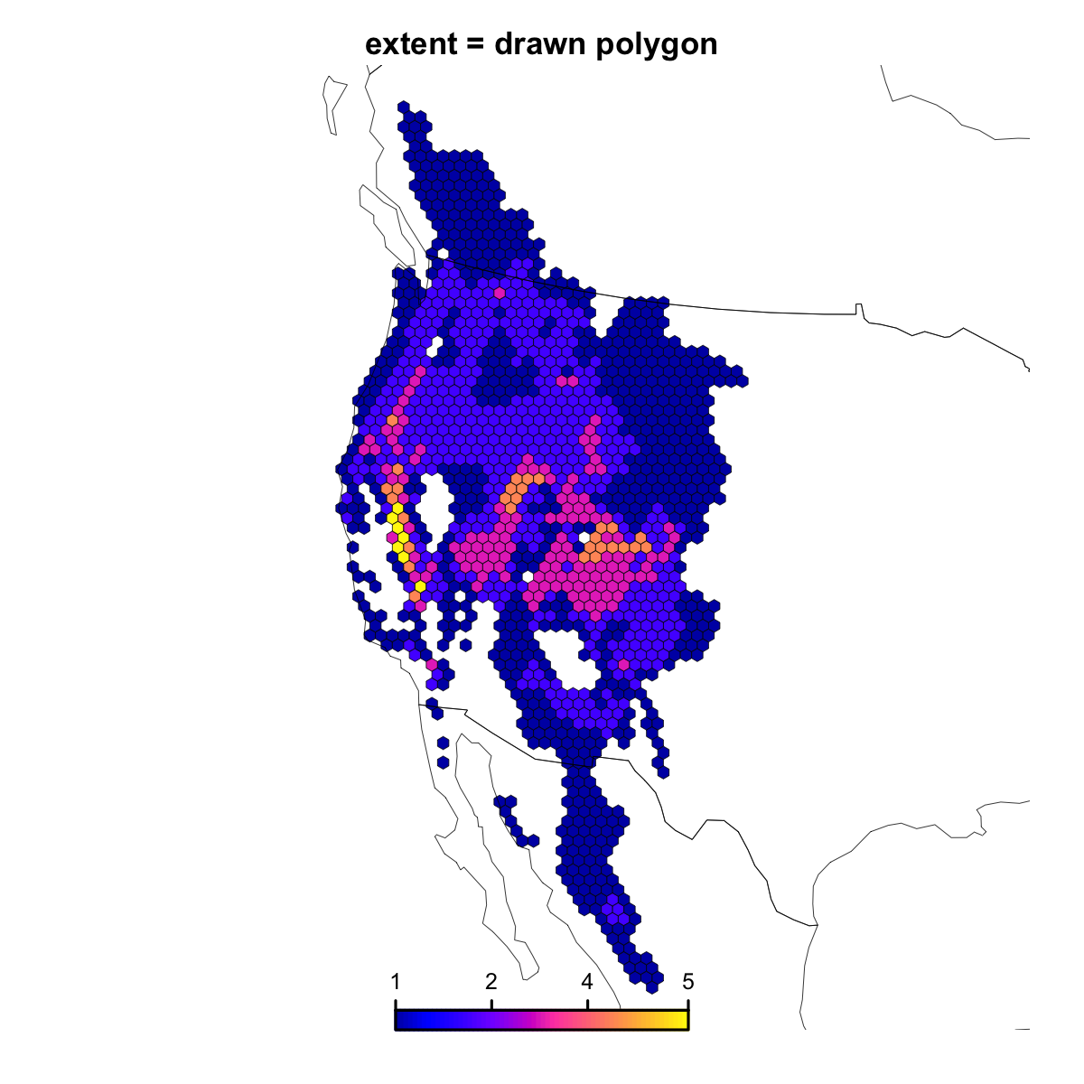
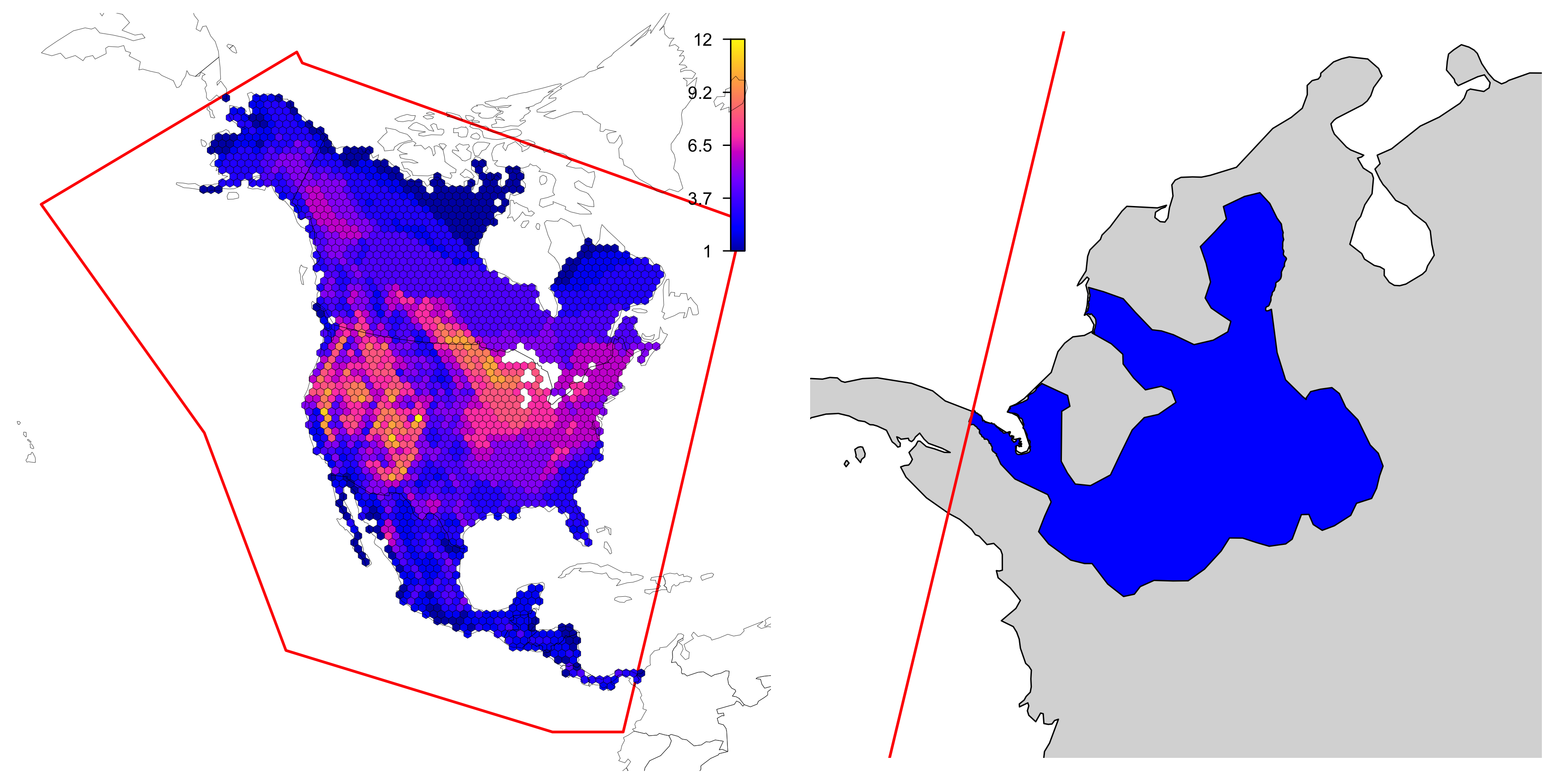
You can optionally enable a filter based on the percent of a species geographic range area that overlaps the specified extent. For instance, if percentWithin = 0.05, then species whose geographic ranges overlap the extent area by < 5% will not be included in the epmGrid object. This can provide a simple way to quickly exclude species whose ranges technically do overlap the region of interest, but that should not functionally be part of the analysis, perhaps because there is a focus on a specific species pool. Use of this filter may or may not make sense, depending on the goals of the analysis.
For instance, in the following example, I've specified my desired extent via the interactive feature. On the left, you can see the resulting epmGrid map and the extent polygon. On the right, you can see the geographic range of a particular species, Microsciurus santanderensis, that got included in the analysis because 0.01% of its geographic range was within the extent polygon. Depending on the application, this may not be desired.
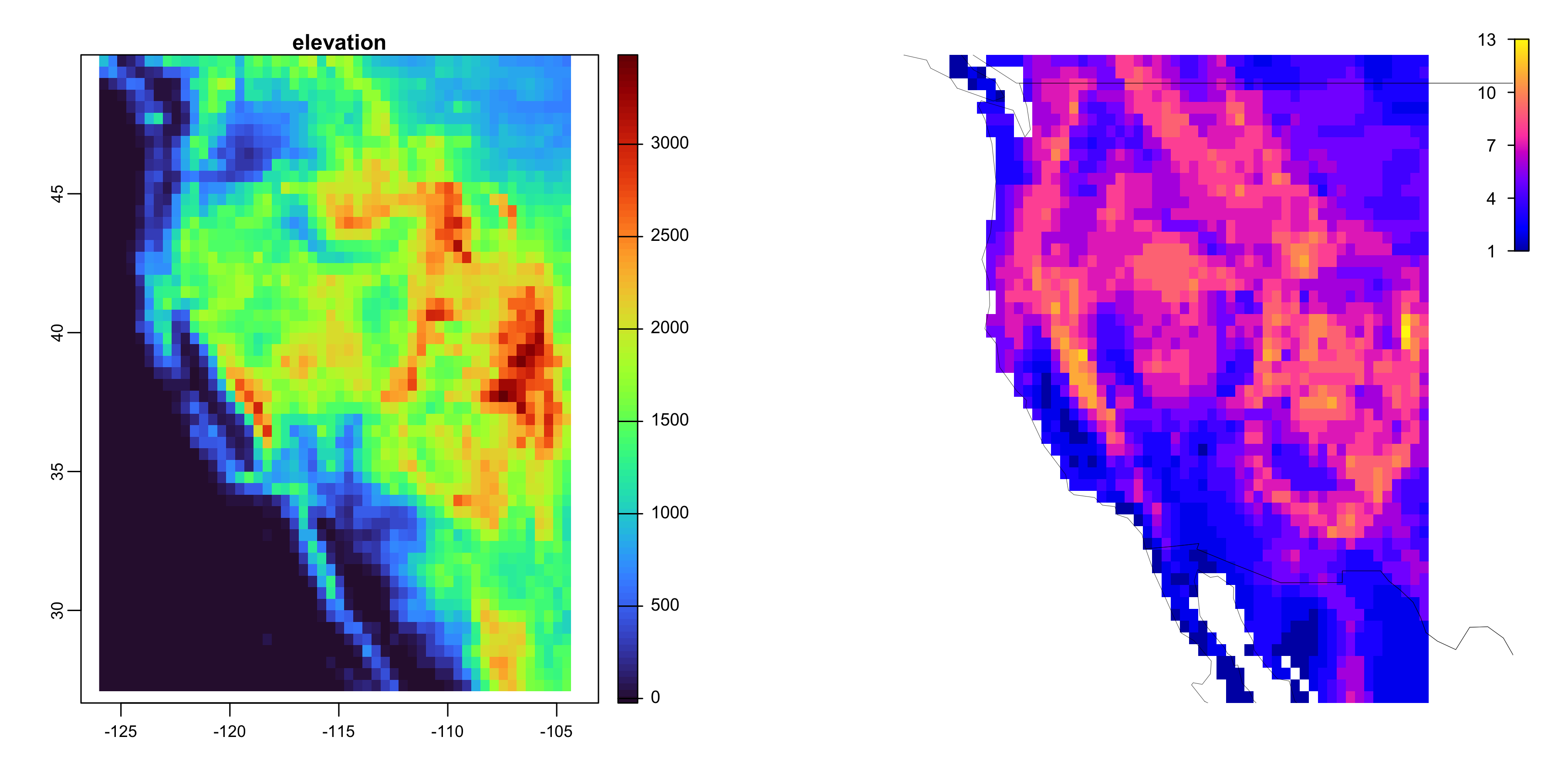
If you have a raster (either RasterLayer via the raster package, or SpatRaster via the terra package), then you can provide it to the template argument, and the resulting epmGrid object will be composed of grid cells that align with that raster. This means that resolution, extent and origin will be derived from that raster, and this will override any other info provided to the extent or resolution arguments.
In the following example, I have an elevation dataset that I provide as a template.
> library(terra)

> elevCrop
class       : SpatRaster
dimensions  : 56, 53, 1  (nrow, ncol, nlyr)
resolution  : 0.4166667, 0.4166667  (x, y)
extent      : -126.0001, -103.9168, 26.66653, 49.99986  (xmin, xmax, ymin, ymax)
coord. ref. : +proj=longlat +datum=WGS84 +no_defs
source      : memory
name        : elev_GMTED2010
min value   :       -24.2752
max value   :       3483.724

xx <- createEPMgrid(spList, cellType = 'square', method = 'centroid', template = elevCrop)

> # are the rasters identical?
> compareGeom(elevCrop, xx[[1]], crs = TRUE, ext = TRUE, rowcol = TRUE, res = TRUE)
[1] TRUE