Creating epmGrid objects
On this page:
- What is an
epmGridobject? - Creating an
epmGridobject from range polygons - A brief description of the options
- Creating the
epmGridobject - Adding trait or phylogenetic data
Link back to the table of contents.
The core R object in the epm package is an object of class epmGrid.
An epmGrid object is a list that contains the following components:
- a grid made up of either hexagonal or square cells
- a list of the unique species communities found in these gridcells
- an indexing vector that links each unique species community to the appropriate gridcells
- a vector of the unique species found throughout the cell communities
- the counts of cells that make up each species' geographic range (for calculating range-weighted metrics)
- ecological / morphological data
- a phylogeny
epmGrid objects can be generated either from species geographic range polygons or from point occurrence records. We will demonstrate how this is done, and what decisions need to be made in choosing from the various options.
We will present the following demonstration based on mammal range polygons downloaded from IUCN, but there are of course a variety of ways you might generate or acquire geographic range polygons for a set of species.
More specifically, we will focus our examples on North American squirrels.
To see a demonstration of how to create an epmGrid object from point occurrences instead of from range polygons, see here.
We will handle spatial data in R using the sf package. However, if you are not as familiar with sf and are more comfortable working SpatialPolygons objects via the sp package, that's ok! An alternative script will be linked below that uses SpatialPolygons rather than sf objects.
> library(sf)
> library(epm)

> # filename and location of IUCN mammals shapefile
> IUCNfile <- "MAMMALS_TERRESTRIAL_ONLY/MAMMALS_TERRESTRIAL_ONLY.shp"

> # load the shapefile as a simple features object
> mammals <- st_read(IUCNfile, stringsAsFactors = FALSE)

Reading layer `MAMMALS_TERRESTRIAL_ONLY' from data source `MAMMALS_TERRESTRIAL_ONLY/MAMMALS_TERRESTRIAL_ONLY.shp' using driver `ESRI Shapefile'
Simple feature collection with 12483 features and 28 fields
Geometry type: MULTIPOLYGON
Dimension:     XY
Bounding box:  xmin: -179.999 ymin: -55.97946 xmax: 179.999 ymax: 83.62744
Geodetic CRS:  WGS 84
The binomial field contains the taxon names. Make sure the taxon field is of mode character and not factor:
> class(mammals$binomial)
[1] "character"
As we are focusing on North American squirrels, we will identify all the relevant species using a bit of regular expression. Here, any taxon names that contains any of the listed terms will be returned (the | implies "or").
> allsp <- unique(mammals$binomial)
> squirrelSp <- grep("Spermophilus\\s|Citellus\\s|Tamias\\s|Sciurus\\s|Glaucomys\\s|Marmota\\s|Cynomys\\s", allsp, value = TRUE, ignore.case = TRUE)
> head(squirrelSp)
[1] "Ammospermophilus nelsoni" "Callosciurus adamsi"      "Callosciurus albescens"
[4] "Callosciurus baluensis"   "Callosciurus caniceps"    "Callosciurus erythraeus"
The mammal ranges are currently all combined into a multipolygon object. We will now extract the squirrel species and store them as a list of separate species range polygons.
> spList <- vector('list', length(squirrelSp))
> names(spList) <- squirrelSp
>
> for (i in 1:length(squirrelSp)) {
+ 	ind <- which(mammals$binomial == squirrelSp[i])
+ 	spList[[i]] <- mammals[ind,]
+ }
Although we won't go into detail here as to the how and why, polygons can potentially have geometry issues -- that is, there may be issues with the topology of the polygons, and this can have undesirable effects downstream. We will demonstrate one way to address this potential problem. Here, we will test each range polygon for problems, and attempt to repair the polygon if need be.
> for (i in 1:length(spList)) {
+ 	if (!any(st_is_valid(spList[[i]]))) {
+ 		message('\trepairing poly ', i)
+ 		spList[[i]] <- st_make_valid(spList[[i]])
+ 	}
+ }
In this case, no issues were detected. Good!
These range polygons are unprojected, in longitude/latitude. We would like to work with equal area grid cells, so we will transform these range polygons to an equal area projection. The North America Albers Equal Area projection works well for North America, so we will use the following coordinate system definition:
> EAproj <- '+proj=aea +lat_1=20 +lat_2=60 +lat_0=40 +lon_0=-96 +x_0=0 +y_0=0 +ellps=GRS80 +datum=NAD83 +units=m +no_defs'
And we will now transform our range polygons.
> spListEA <- lapply(spList, function(x) st_transform(x, st_crs(EAproj)))
We will also make some changes to some of the taxonomy so that it matches with taxonomic and phylogenetic data later on.
names(spList) <- gsub('Neotamias', 'Tamias', names(spList))
names(spListEA) <- gsub('Neotamias', 'Tamias', names(spListEA))

# Replace all spaces with underscores (not strictly necessary, but this will match the phylogenetic data later on)
names(spList) <- gsub('\\s+', '_', names(spList))
names(spListEA) <- gsub('\\s+', '_', names(spListEA))
At this stage, we have range polygons for 187 squirrel species and we are ready to use the epm package. Click here to see R code that does the same thing as above, but with SpatialPolygons and the sp package, rather than the sf package.
The function createEPMgrid() will take range polygons and create an epmGrid object.
This involves a number of options to consider. We will list the arguments in createEPMgrid() and briefly explain what options there are to choose from. You will find further demonstrations of the different options elsewhere on this wiki.
resolution: We need to choose the size of the gridcells. The nature of the input data and the purpose of the research will dictate what a reasonable resolution should be. Importantly, resolution is in the spatial units of the input data. As we projected our range polygons to an equal area projection, units are meters. We will set the resolution to 50km (= 50000 m).
method: There are two options for determining whether a species range polygon should register in a given grid cell. With method 'centroid', a range polygon registers if it intersects the centroid coordinates of the grid cell. With method 'percentOverlap', a range polygon registers for a given cell if it covers xx% of that cell, where xx is supplied via the 'percentThreshold' input argument. More details can be found here.
cellType: We can choose between hexagonal and square grid cells. Hexagonal grid cells are preferable for several reasons:
- Each cell has a clear set of 6 neighboring cells, which is good for turnover metrics,
- hexagonal grids can more naturally follow contours and irregular shapes and provide nice map aesthetics, and
- if working with unprojected data, hexagonal grid cells can be of different sizes.
On the other hand, square grid cell might be preferable if you are working at a very high spatial resolution, as raster data storage is more efficient. Square grid cells might also be preferable if you intend to work with other raster datasets, such that the grid cells align.
Some of these differences can be seen in the graphic associated with the first extent example.
retainSmallRanges: an option where if a species has a range that is smaller than a single grid cell, it might get dropped because it registers nowhere (either because it does not overlap any cell midpoint coordinates or because it occupies too little of any cell's area). If this option is set to TRUE, then the species will still register in the cell that it most occupies. More details can be found here.
extent: The extent of the epmGrid object can be specified a number of ways:
- If
extent = 'auto', then the full extent of the input data will be used. - If
extentis a polygon, then the returned object will be cropped and masked to that polygon. - You can also supply
c(minX, maxX, minY, maxY)as the x and y ranges for cropping. - Finally, if
extent = 'interactive', then a map will be displayed where you can define a polygon by hand. The selected polygon will be returned by the function so that you can copy/paste it as a polygon supplied to the extent argument in a subsequent call to the function. More details can be found here.
template: As an alternative to the 'resolution' and 'extent' arguments, you can provide a raster as a template, and resolution and extent will be derived from that raster. Useful if you are trying to match the spatial configuration of another dataset. More details can be found here.
percentWithin: This is an optional filter that will calculate the percent of each species' range that is within the analysis extent, and will exclude species if the percent area is below this threshold. More details can be found here.
Now that we've seen a brief explanation of the available options, we will now create an epmGrid object. We will set the resolution to 50km, we will opt to retain small-ranged species that would otherwise be lost, we will use hexagonal cells.
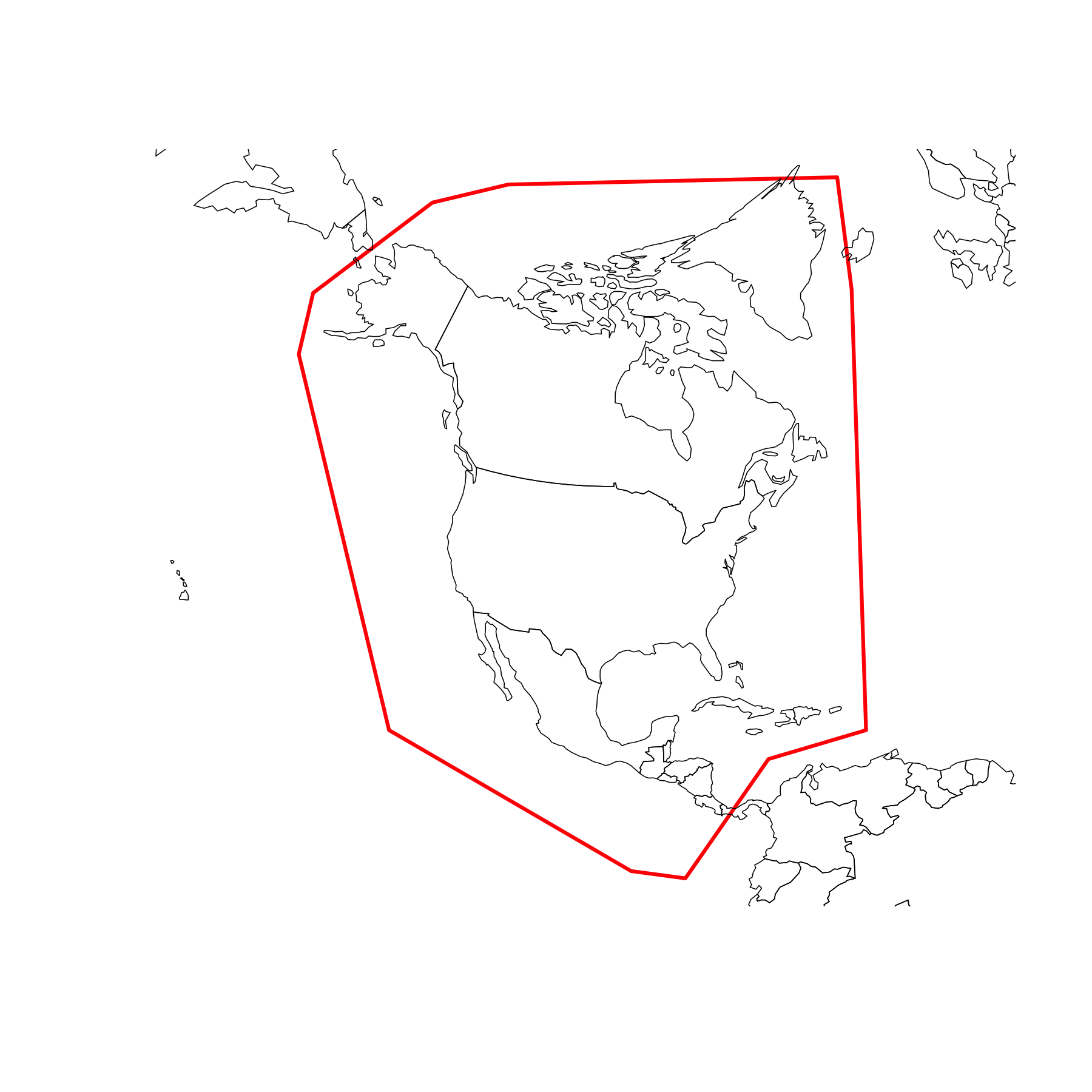
First, let's use the interactive extent drawing feature. We'll also provide some bounds since it's hard to draw an extent for a global dataset:
extentPoly <- createEPMgrid(spListEA, resolution = 50000, retainSmallRanges = TRUE, extent = list('interactive', c(-5e+06, 5e+06, -5e+06, 5e+06)), method = 'centroid', cellType = 'hex')
This has returned the polygon that was drawn, in wkt format.
> extentPoly
[1] "POLYGON ((-2906193 4690015, -3110223 4376122, -3377032 4172092, -3769399 3873894, -4083291 3340276, -4067597 2728184, -2702163 -1509370, 782048.5 -4036208, 1425529 -3973429, 1802200 -3785093, 2163177 -2639384, 3622779 -2027293, 2900826 5396274, 578018.1 5207938, -2906193 4690015))"
Let's plot it.
plot(st_as_sfc(extentPoly, crs = st_crs(spListEA[[1]])), lwd = 2, border = 'red')
plot(st_transform(epm:::worldmap, crs = st_crs(spListEA[[1]])), add = TRUE, lwd = 0.5)
So that we can rerun this code in the future and use the same extent, let's copy/paste it here.
extentPoly <- "POLYGON ((-2906193 4690015, -3110223 4376122, -3377032 4172092, -3769399 3873894, -4083291 3340276, -4067597 2728184, -2702163 -1509370, 782048.5 -4036208, 1425529 -3973429, 1802200 -3785093, 2163177 -2639384, 3622779 -2027293, 2900826 5396274, 578018.1 5207938, -2906193 4690015))"
We will now run the function again, but this time provide the extent polygon.
> squirrelEPM <- createEPMgrid(spListEA, resolution = 50000, retainSmallRanges = TRUE, extent = extentPoly, method = 'centroid', cellType = 'hex')
  |++++++++++++++++++++++++++++++++++++++++++++++++++| 100% elapsed=02m 53s
3 small-ranged species were preserved:
	Marmota_vancouverensis
	Tamiasciurus_mearnsi
	Urocitellus_brunneus

100 species are being dropped.

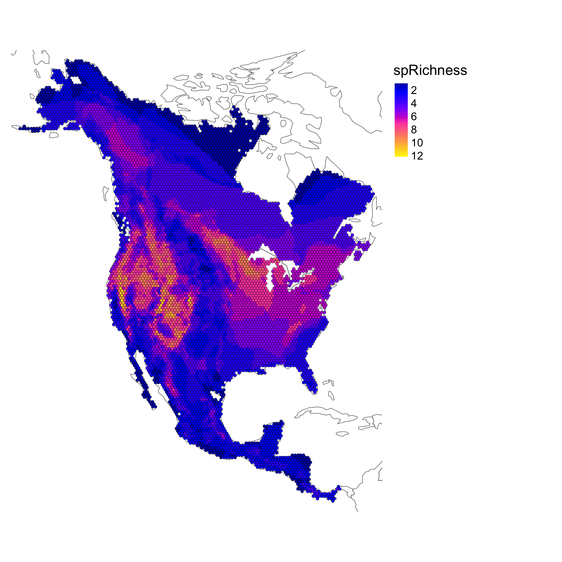
> plot(squirrelEPM)
We can see a quick summary of the epmGrid object
> squirrelEPM

	Summary of epm object:

	metric: spRichness
	grid type:  hexagon
	number of grid cells: 9063
	grid resolution: 50000 by 50000
	projected: TRUE
	crs: +proj=aea +lat_1=20 +lat_2=60 +lat_0=40 +lon_0=-96 +x_0=0 +y_0=0 +ellps=GRS80 +datum=NAD83 +units=m +no_defs

	number of unique species: 87 (richness range: 1 - 12)
	data present: No
	phylogeny present: No
This tells us that this epmGrid object's primary metric is species richness (since we haven't done any morphological or phylogenetic analyses yet). We can see that we are using hexagonal grid cells, we are shown the resolution and the projection information. We have not yet added any morphological or phylogenetic data.
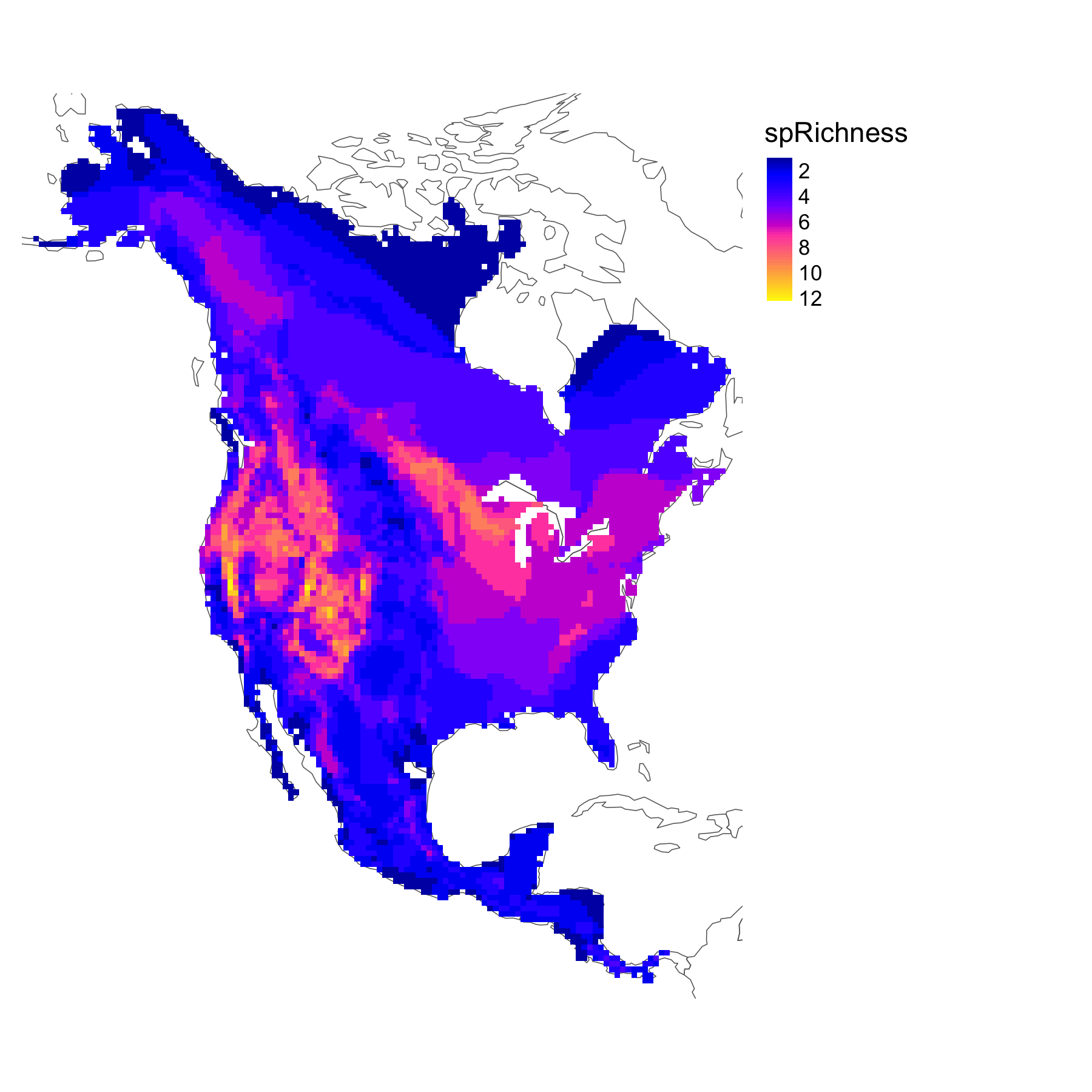
Let's also create an epmGrid object with square grid cells for comparison.
> squareEPM <- createEPMgrid(spListEA, resolution = 50000, retainSmallRanges = TRUE, extent = extentPoly, method = 'centroid', cellType = 'square')
  |++++++++++++++++++++++++++++++++++++++++++++++++++| 100% elapsed=13s
2 small-ranged species were preserved:
	Marmota_vancouverensis
	Urocitellus_brunneus

100 species are being dropped.

> plot(squareEPM)
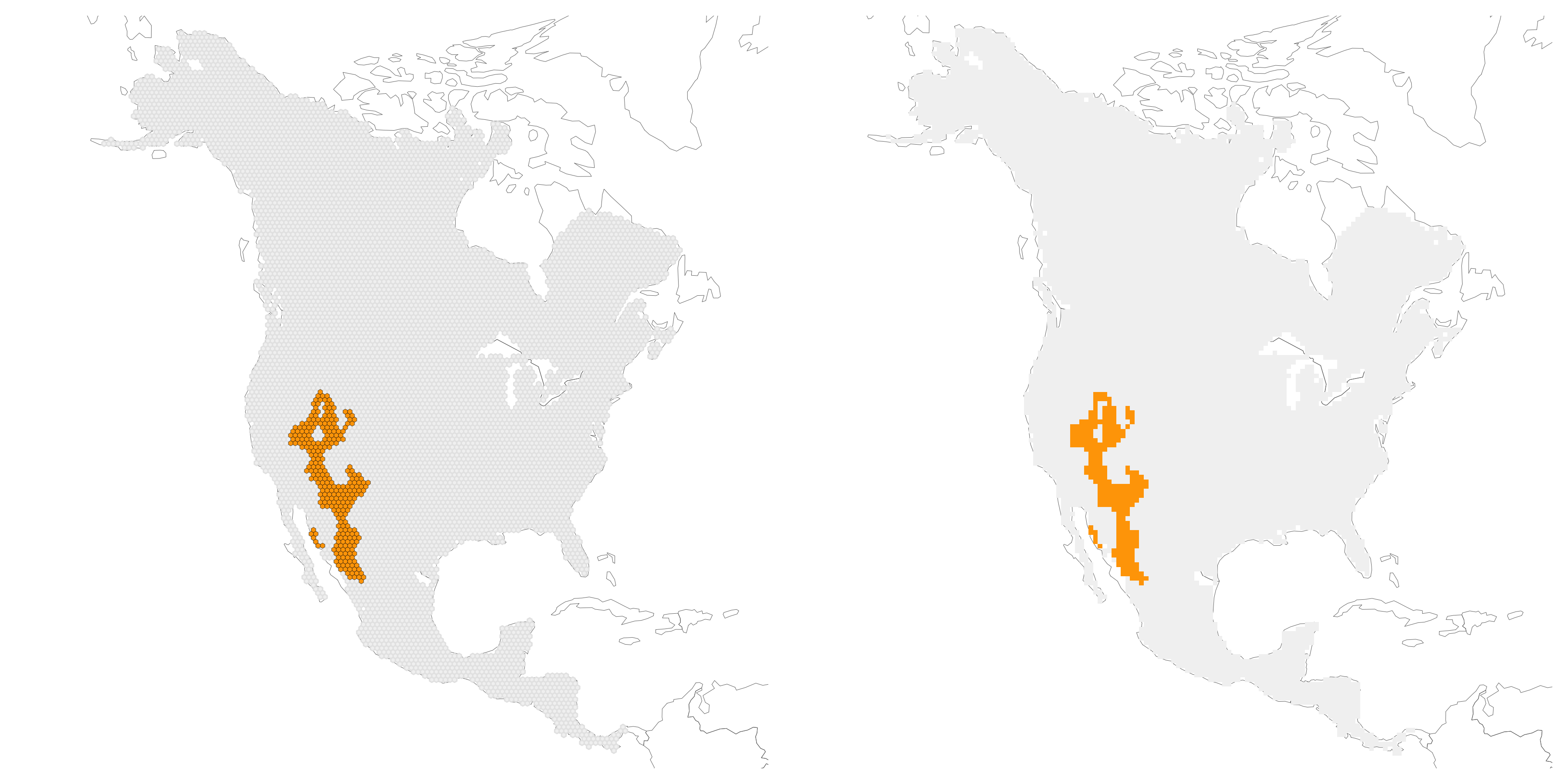
We can also see how a particular species is encoded in the epmGrid object. This can be helpful for confirming that this worked as expected.
map1 <- plotSpRange(squirrelEPM, taxon = 'Tamias_dorsalis', lwd = 0.2)
map2 <- plotSpRange(squareEPM, taxon = 'Tamias_dorsalis')
tmap::tmap_arrange(map1, map2)
Now that we've created our epmGrid object, we can add additional data, such as trait data and/or a phylogeny.
The epm package allows us to add a phylogeny (or multiple phylogenies) to the epmGrid object, in the form of a tree of class phylo.
In terms of trait data, 3 options are possible:
- a single named vector (univariate data)
- a table with traits as columns (species names as rownames)
- a pairwise distance matrix (species names as row and column names)
Here, we will read in a phylogeny and morphometric dataset for squirrels. We will use the ape package for phylogeny handling.
> library(ape)

> tree <- read.nexus('consensus_130528.nex')
> traits <- read.csv('Species_,means_Shape_nexusNames.csv', stringsAsFactors = FALSE, row.names = 1, header = FALSE)

> tree
Phylogenetic tree with 193 tips and 192 internal nodes.

Tip labels:
  Aplodontia_rufa, Glis_glis, Graphiurus_murinus, Muscardinus_avellanarius, Sciurus_niger, Sciurus_griseus, ...

Rooted; includes branch lengths.

> traits[1:10, 1:5]
                                   V2          V3         V4          V5         V6
Aeretes_melanopterus       -0.1472243 -0.02351242 -0.1402814 0.008184952 -0.1132772
Aeromys_tephromelas        -0.1495352 -0.03046051 -0.1537216 0.003249341 -0.1177951
Ammospermophilus_harrisii  -0.1525632 -0.02365629 -0.1626861 0.013549929 -0.1186071
Ammospermophilus_interpres -0.1533976 -0.02345726 -0.1652115 0.017189084 -0.1229425
Ammospermophilus_leucurus  -0.1522449 -0.02332345 -0.1642354 0.013643174 -0.1208897
Atlantoxerus_getulus       -0.1466143 -0.02463764 -0.1589840 0.015588087 -0.1151848
Belomys_pearsonii          -0.1537330 -0.02435239 -0.1560778 0.007216735 -0.1143427
Callosciurus_caniceps      -0.1389825 -0.03543532 -0.1626198 0.012463660 -0.1113677
Callosciurus_erythraeus    -0.1408538 -0.03136944 -0.1578735 0.013161121 -0.1159358
Callosciurus_finlaysonii   -0.1314674 -0.03686896 -0.1600718 0.011931661 -0.1171905
It is critical that the same taxonomy be applied to all datasets, otherwise species will be dropped, or assigned to the wrong data. Here, we will apply the same synonymy changes so that these data match our geographic range data.
> rownames(traits) <- gsub('^Neotamias', 'Tamias', rownames(traits))
> tree$tip.label <- gsub('^Neotamias', 'Tamias', tree$tip.label)

> rownames(traits) <- gsub('\\s+', '_', rownames(traits))
> tree$tip.label <- gsub('\\s+', '_', tree$tip.label)

# How many species are shared between our geographic data and our trait or phylo data?
> length(intersect(rownames(traits), names(spListEA)))
[1] 116
> length(intersect(tree$tip.label, names(spListEA)))
[1] 131
We can now add these datasets to the epmGrid object. Because the trait and phylo datasets contain more species than just the North American squirrel species that we have in our epmGrid object, only overlapping species will be kept.
> squirrelEPM <- addTraits(squirrelEPM, traits)
Warning message:
In addTraits(squirrelEPM, traits) :
  99 species were dropped from the trait data because they lack geographic data.

> nrow(traits)
[1] 168
> squirrelEPM <- addPhylo(squirrelEPM, tree)
Warning message:
In addPhylo(squirrelEPM, tree) :
  122 species were pruned from the phylogeny because they lack geographic data.
And now when we look at the summary, we should see these new additions.
> squirrelEPM

	Summary of epm object:

	metric: spRichness
	grid type:  hexagon
	number of grid cells: 9063
	grid resolution: 50000 by 50000
	projected: TRUE
	crs: +proj=aea +lat_1=20 +lat_2=60 +lat_0=40 +lon_0=-96 +x_0=0 +y_0=0 +ellps=GRS80 +datum=NAD83 +units=m +no_defs

	number of unique species: 87 (richness range: 1 - 12)
	data present: Yes
	number of species shared between data and grid: 69
	phylogeny present: Yes
	number of species shared between phylogeny and grid: 71
When adding trait data to an epmGrid object, only trait taxa that already exist in the epmGrid object are kept, and similarly, only taxa shared between the epmGrid object and a phylogeny are kept when adding in a tree. However, this means that the epmGrid object may contain information for taxa that are not shared across the trait and phylogenetic datasets.
If it is important to have only the set of taxa that are common across all datasets, we can do the following:
> reduceToCommonTaxa(squirrelEPM)

	Summary of epm object:

	metric: spRichness
	grid type:  hexagon
	number of grid cells: 8849
	grid resolution: 50000 by 50000
	projected: TRUE
	crs: +proj=aea +lat_1=20 +lat_2=60 +lat_0=40 +lon_0=-96 +x_0=0 +y_0=0 +ellps=GRS80 +datum=NAD83 +units=m +no_defs

	number of unique species: 69 (richness range: 1 - 12)
	data present: Yes
	number of species shared between data and grid: 69
	phylogeny present: Yes
	number of species shared between phylogeny and grid: 69
You can see that now there are fewer taxa that are shared between the phylogeny and the grid, and importantly, only taxa that have all data types are retained.