Spectral Analysis of Lung Sounds for Asthma & Pneumonia Classification

Figure 1. Proposed Methodology (extracted from IEEE paper)

📖 Overview

This repository accompanies the IEEE conference paper:

“Spectral Analysis of Lungs sounds for Classification of Asthma and Pneumonia Wheezing” (ICECCE 2025, Istanbul, Turkey).

Lung sounds provide critical diagnostic information. Wheezing is a key indicator of pulmonary illnesses such as Asthma and Pneumonia. This project presents a complete ML pipeline — from preprocessing raw lung sounds, to spectral feature extraction, and classification via Support Vector Machine (SVM) with an accuracy of 96.7%.

Python Code Implementation Video:

Part 1

Part 2

Part 3

---

IEEE Paper Explained

---

ICECCE Paper Presentaion Video

📂 Repository Contents

• paper/ → Full IEEE paper (PDF)
• notebooks/ → Jupyter/Kaggle notebooks for preprocessing, feature extraction & classification
• gui_app/ → Ready-to-deploy GUI (lungsound_gui.py)
• data/ → Example lung sound samples (optional small demo files)
• results/figures/ → Extracted figures and generated plots

⚙️ Environment Setup

We recommend using Anaconda.

# Create environment
conda env create -f environment.yml
conda activate lungsound-env

Key libraries: numpy, scipy, librosa, matplotlib, scikit-learn, tkinter.

🛠️ How to Run

---

1) Preprocessing

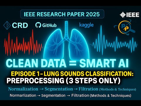
Open notebooks/preprocessing.ipynb in Jupyter/Kaggle. It demonstrates:

• Normalization (Min–Max scaling)
• Segmentation (250 ms frames)
• Butterworth bandpass filtering (250 Hz – 2 kHz)

📌 Overview

This notebook focuses on preprocessing lung sound recordings for respiratory disease classification.
The workflow consists of three key stages:

1. Normalization – removing amplitude variations.
2. Segmentation – dividing signals into frames.
3. Filtration – applying band-pass filtering to isolate useful frequency bands.

The processed signals are later used for feature extraction and classification of respiratory conditions such as Normal, Asthma, and Pneumonia.

🎚 Step 1: Band-pass Filtering

To remove unwanted low- and high-frequency components, a 10th-order Butterworth band-pass filter was applied.
This retains only frequencies between 150 Hz – 2000 Hz, where most lung sound information lies.

📏 Step 2: Dimension & Framing Report

Input signals were preprocessed and segmented into overlapping frames:

• Sampling rate: 44.1 kHz
• Frame length: 0.25s (11025 samples)
• Hop size: 0.125s (5512 samples, 50% overlap)

Frames with silence were removed, leaving ~80% of useful frames.

🫁 Step 3: Preprocessed Lung Sounds (Overlay)

Signals for different classes (Normal, Asthma, Pneumonia) after preprocessing, plotted in the time domain.

Similarly, in the frequency domain we observe different spectral patterns among the classes.

📊 Step 4: Class-wise Visualization

Time Domain (per class)

• Normal: Clear periodic bursts.
• Asthma: Weak, noisy signal with irregular patterns.
• Pneumonia: Distorted and suppressed signal structure.

Frequency Domain (per class)

Each respiratory condition shows a distinct spectral signature:

• Normal: Strong low-frequency energy.
• Asthma: Broader spread with weaker energy.
• Pneumonia: Different high-frequency attenuation.

✅ Summary

The preprocessing pipeline ensures that lung sound signals are:

• Normalized to remove amplitude variations.
• Segmented into meaningful frames.
• Filtered to retain medically relevant frequency ranges.

This structured approach lays the foundation for robust feature extraction and classification in later stages.

---

2) Feature Extraction

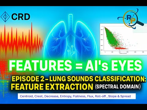
We extract nine spectral features: Spectral Centroid, Spectral Crest, Spectral Decrease, Spectral Entropy, Spectral Flatness, Spectral Flux, Spectral Roll‑off, Spectral Slope, Spectral Spread.

📌 Overview

This notebook extends the preprocessing pipeline by extracting meaningful features from lung sound recordings.
Feature extraction bridges the gap between raw signals and machine learning models, enabling accurate classification of respiratory conditions (Normal, Asthma, Pneumonia).

The workflow covers:

1. Time-domain features
2. Frequency-domain features
3. Spectral descriptors

⚙️ Processing Status

The dataset was processed class-wise, with 100% completion for all categories.

---

📑 Extracted Features

Each audio frame was characterized using spectral descriptors, including:

• SCN: Spectral Centroid
• SCR: Spectral Crest
• SDC: Spectral Decrease
• SEN: Spectral Entropy
• SFL: Spectral Flatness
• SFLUX: Spectral Flux
• SRO: Spectral Roll-off
• SSL: Spectral Slope
• SSP: Spectral Spread

Example snapshot of extracted features:

📊 Feature Visualization

SCN vs SCR

Demonstrates how Spectral Centroid relates to Spectral Crest, differentiating lung conditions.

SCN vs SEN

Shows correlation between Spectral Centroid and Spectral Entropy, highlighting Asthma’s distinct pattern.

SCN vs SFLUX

Visualizes spectral fluctuations and their distribution across conditions.

🔗 Feature Correlations

Understanding inter-feature dependencies is crucial for model selection and dimensionality reduction.

• Overall correlation (all classes):
  Strong correlations between SCN, SDC, SEN, and SRO.

• Class-wise correlations:

Normal

Asthma

Pneumonia

✅ Summary

• Extracted time-domain, frequency-domain, and spectral features.
• Demonstrated feature separability across conditions via scatter plots.
• Analyzed feature correlations to guide further dimensionality reduction and classification.

This feature set forms the foundation for Notebook 3: Feature Selection & Classification.

---

3) Classification

📌 Overview

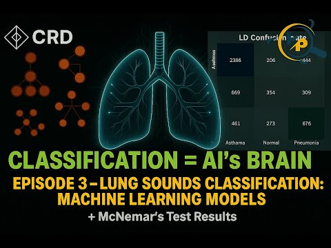
This notebook demonstrates the classification of respiratory conditions (Normal, Asthma, Pneumonia) using spectral features extracted in Notebook 2.
Multiple machine learning algorithms are applied, and their performance is evaluated using confusion matrices, accuracy, precision, recall, F1-score, and statistical significance testing.

📊 Dataset Split

The dataset was divided into training and testing sets:

• Training samples: 14,879
• Testing samples: 6,378

🧠 Classifiers Evaluated

The following models were tested:

1. LD – Linear Discriminant
2. KNB – Kernel Naïve Bayes
3. FT – Fine Tree
4. GNB – Gaussian Naïve Bayes
5. FKNN – Fine K-Nearest Neighbors
6. BT – Bagged Trees
7. SKNN – Subspace K-Nearest Neighbors

📉 Confusion Matrices

Confusion matrices illustrate the classification performance of each model.

• LD
  

• KNB
  

• FT
  

• GNB
  

• FKNN
  

• BT
  

• SKNN
  

📑 Performance Metrics

Performance of each classifier was evaluated with Accuracy, Precision, Recall, and F1-score.

Accuracy Comparison

F1-Score Comparison

📊 Statistical Significance Testing

To ensure differences in classifier performance are not due to chance, McNemar’s Test was applied.

🔎 McNemar’s Test vs SVM

All models showed statistically significant differences compared to SVM at 95% confidence.

🔎 McNemar’s Test vs FT (Fine Tree)

Fine Tree was compared against all other models, and the results confirm its superiority with statistically significant differences.

---

✅ Summary & Insights

• Best Performing Models:
  • Bagged Trees (BT) and Fine Tree (FT) achieved the highest accuracy (~98%) and F1-scores (~0.97–0.98).
• Moderate Performance:
  • FKNN and SKNN scored ~85% accuracy and F1 ~0.82.
• Weaker Performance:
  • LD, KNB, GNB underperformed (<65% accuracy, low F1).
• Statistical Testing:
  • Confirmed FT and BT significantly outperform other models.

📌 Conclusion:
Tree-based ensemble methods (BT, FT) provide the most reliable classification of lung sounds, with results statistically validated using McNemar’s Test.

---

4) GUI Application 🎛️

Run the GUI app to classify any .wav lung sound file:

conda activate lungapp
streamlit run gui_app/spectral-lungsound-gui.py

Features:

• Load lung sound file

• View preprocessing plots and timing

• Extract and visualize features

• Run trained models

• Display final classification (Asthma / Pneumonia / Normal) with metrics

  

📜 Reference

@inproceedings{naqvi2020spectral, title={Spectral analysis of lungs sounds for classification of asthma and pneumonia wheezing}, author={Naqvi, Syed Zohaib Hassan and Arooj, Misha and Aziz, Sumair and Khan, Muhammad Umar and Choudhary, Mohammad Ahmad and others}, booktitle={2020 International Conference on Electrical, Communication, and Computer Engineering (ICECCE)}, pages={1--6}, year={2020}, organization={IEEE} }

---

This repository is designed as an educational resource for students and researchers in Biomedical Engineering & Signal Processing.